Wednesday, November 22, 2006

SnapDrive for Unix: Self Service Storage Management

I was reading an article recently regarding Storage provisioning, the article was titled “The Right Way to Provision Storage”. What I took away from the article, as reader, is that storage provisioning is a painful, time consuming process involving several people representing different groups.

The process according to the article pretty much goes like this:

Step 1: DBA determines performance requirement and number of LUNs and defers to the Storage person
Step 2: Storage person creates the LUN(s) and defers to the Operations person
Step 3: Operations person maps the LUN(s) to some initiator(s) and defers to the Server Admin
Step 4: Server Admin discovers the LUN(s) and creates the Filesystem(s). Then he/she informs the DBA, probably 3-4 days later, that his/her LUN(s) are ready to host the application

I wonder how many requests per week these folks get for storage provisioning and how much of their time it consumes. I would guess, much more than they would like. An IT director of a very large and well know Financial institution, a couple of years ago, told me “We get over a 400 storage provisioning requests a week and it has become very difficult to satisfy them all in a timely manner”.

Why does storage provisioning have to be so painful? It seems to me that one would get more joy out of getting a root canal than asking for storage to be provisioned. Storage provisioning should be a straight forward process and the folks who own the data (Application Admins) should be directly involved in the process.

In fact, they should be the ones doing the provisioning directly from the host under the watchful eye of the Storage group who will control the process by putting the necessary controls in place at the storage layer restricting the amount of storage Application admins can provision and the operations they are allowed to perform. This would be self-service storage provisioning and data management.

Dave Hitz on his blog, a few months back, described the above process and used the ATM analogy as example.

NetApp’s SnapDrive for Unix (Solaris/AIX/HP-UX/Linux) is similar to an ATM. It lets data application admins manage and provision storage for the data they own. Thru deep integration with various Logical Volume Managers, filesystem specific alls, SnapDrive for Unix allows administrators to do the following with a single host command:

1) Create LUNs on the array
2) Map the LUNs to host initiators
3) Discover the LUNs on the host
4) Create Disk Groups/Volume Groups
5) Create Logical Volumes
6) Create Filesystems

7) Add LUNs to Disk Group
8) Resize Storage
9) Create and Manage Snapshots
10) Recover from Snapshots
11) Connect to filesystems in Snapshots and mount them onto the same or a different Host the original filesystem was or still is mounted

The whole process is fast and more importantly very efficient. Furthermore, it masks the complexity of the various UNIX Logical Volume Managers and allows folks who are not intimately familiar with them to successfully perform various storage related tasks.

Additionally, SnapDrive for Unix provides snapshot consistency by making calls to filesystem specific freeze/thaw mechanisms providing image consistenty and the ability to successfully recover from a Snapshot.

Taking this a step further, SnapDrive for Unix provides the necessary controls at the storage layer and allows Storage administrators to specify who has access to what. For example, an administrator can specify any or a combination of the following access methods.

NONE − The host has no access to the storage system.
◆ CREATE SNAP − The host can create snapshots.
◆ SNAP USE − The host can delete and rename snapshots.
◆ SNAP ALL− The host can create, restore, delete, and rename
snapshots.
◆ STORAGE CREATE DELETE − The host can create, resize,
and delete storage.
◆ STORAGE USE − The host can connect and disconnect storage.
◆ STORAGE ALL − The host can create, delete, connect, and
disconnect storage.
◆ ALL ACCESS− The host has access to all the SnapDrive for
UNIX operations.

Furthermore, SnapDrive for Unix is tightly integrated with NetApp’s SnapManager for Oracle product on several Unix platforms which allows application admins to manage Oracle specific Datasets. Currently, SnapDrive for Unix supports Fibre Channel, iSCSI and NFS.

SnapDrive for Unix uses HTTP/HTTPs as a transport protocol with password encryption and makes calls to DataONTAP’s APIs for storage management related tasks.

There’s also a widely deployed Windows version of SnapDrive that integrates with Microsoft’s Logical Disk Manager/NTFS and VSS and allows admins to perform similar tasks. Furthermore, SnapDrive for Windows is tightly integrated with NetApp’s SnapManager for Exchange and SnapManager for SQL products that allow administrators to obtain instantaneous backups and near-instantaneous restores of their Exchange or SQL server database(s).

Below are a couple of examples from my lab server of using SnapDrive for Unix of what it takes to provision Storage on a Solaris host with Veritas Foundation Suite installed.

Example 1:

In this example I’m creating 2 LUNs of 2GB size each on controller named filer-a on volume named /vol/boot.
The LUNs are named lun1 and lun2. I then create a Veritas disk group named dg1. On that disk group I create a Veritas volume named testvol. On volume testvol, I then create a filesystem with /test as the mount point. By default and unless instructed otherwise via a nopersist option, SnapDrive will also make an entries into the Solaris /etc/vfstab file.

The following is what the filesystem looks like and Veritas sees immidiately after the above process has completed:


Example 2:

Below, I obtain a snapshot of the Veritas filesystem and name the snapshot test_snap. I then make an inquiry to the array to obtain a list of consistent snapshots for my /test filesystem.

This reveals that I have taken 3 different snapshots at different points in time and I can recover from anyone of them. I can also connect to any one of them and mount the filesystem.
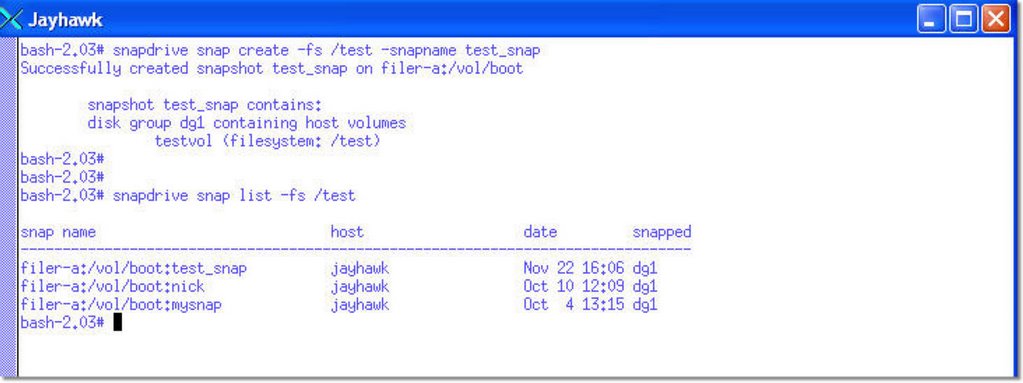


Example 3

Here I'm connecting to the filesystem from the most recent snapshot, test_snap, and i'm mounting a space optimized clone of the original filesystem at the time the snapshot was taken. Ultimately, I will end up with 2 copies of the filesystem.
The original one, named /test, and the one from the snapshot which I will rename /test_copy. Both of the filesystems are mounted on the same Solaris server (they don't have to be) and are under Veritas Volume Manager control.

This is how simple and easy it is to provision and manage storage using NetApp's SnapDrive. Franky, it seems to be that a lengthy process explaining the "proper" way to provision storage adds extra layers of human intervention, uncessary complexity, it's inefficient and time consuming.


Thursday, September 14, 2006

The Emergence of OS Native Multipathing Solutions

In today’s Business environment, High Availability is not an option. It is a business necessity and is essential in providing Business Continuity. Data is the lifeblood of a Business. Can you imagine a financial firm loosing connectivity to its Business Critical Database in the middle of the day?

This is where Multipathing or Path failover solutions can address High Availability and Business Continuity because not only do they eliminate single points of failure between the server and the storage but also help in achieving better performance by balancing the load (I/O load or LUN load) across multiple paths.

Most new servers bought today by customers connect into SANs. Furthermore, most of these servers have high availability and redundancy requirements thus are connecting to highly available, redundant fabrics and disk arrays. When any component in the data path fails, failover to the surviving data path occurs non-disruptively and automatically.
So the premise of Multipathing or path failover is to provide redundant server connections to storage and:
  • Provide path failover in the event of a path failure
  • Monitor I/O paths and provide alerts on critical events


Over the years, administrators have recognized this need and so after the purchase of a server, they would also purchase a 3rd party multipathing solution, typically from their storage vendor. Apart from the fact that these 3rd party solutions were not designed as part of Operating System and some did not integrate particularly well, in addition, they did not interoperate well with multipathing solutions from other storage vendors that needed to installed on the same server. In essence, storage vendor specific multipathing solutions solved one problem while creating another one. This problem has lasted for years and was addressed only recently.


Over the past 2-3 years a flurry of OS native multipathing solutions have emerged. Thus, today’s multipathing solution distribution model has changed drastically. Multipathing solutions can be distributed either as:

  • 3rd party software (Symantec/Veritas DMP, PowerPath, HDLM, SDD, RDAC, SANPath etc).
  • Embedded in the Operating System (Solaris MPxIO, AIX MPIO, Windows MPIO, Linux Device Mapper-Multipath, HP-UX PVLinks, VMware ESX Server, Netware via NSS).
  • As an HBA vendor device driver that works with most, if not all, storage arrays (i.e Qlogic’s Linux/Netware failover driver, Windows QLDirect)
  • As an HBA vendor device driver (Emulex MultiPulse) available to OEMs only who in turn incorporate the technology into their own products via calls made to the HBA APIs provided by the HBA vendor.


Increasingly, the trend is toward the deployment of OS native multipathing solutions. In fact, with the exception of one Operating System, a substantial server/storage vendor has all but abandoned support of their traditional Multipathing solution for their newer storage arrays, in favor of the OS native ones.

There are two drivers behind this trend. Cost is one reason customers elect to deploy OS native multipathing solutions. After all, you can’t beat “free”. A secondary, but equally important, driver is to achieve better interoperability among various vendors’ storage devices that happen to provision the same server(s). One driver stack and one set of HBAs talks to everybody.

From a Windows standpoint, it is important to note that Microsoft is strongly encouraging all storage vendors to support its MPIO specification. Network Appliance supports this specification with a Device Specific Module (DSM) for our disk subsystems. It’s equally important to note that Windows MPIO enables the co-existence of multiple storage vendor DSMs within the same server. In fact, the current approach is similar to what Symantec/Veritas has done over the years with the Array Support Library (ASL) that provides vendor disk subsystem attributes and multipathing information to the Symantec/Veritas Device Discovery Layer (DDL) and Dynamic Multipathing (DMP) components.

Early last year Microsoft indicated they were considering the development of a Generic DSM for Fibre Channel (Generic DSM for iSCSI already exists) that will support all storage vendors as long as they (storage vendors) comply with the SCSI Primary Commands revision 3 (SCP-3). Furthermore, Microsoft, at the time, indicated that a Generic DSM would be incorporated into the Windows Vista release.

Network Appliance’s primary multipathing approach is to support all OS native multipathing solutions, as well as, support some popular 3rd party (i.e Symantec/VxDMP) solutions across all supported Operating Systems. Depending on customer demand, certification with disk array vendor specific multipathing solutions is always a possibility, assuming the necessary Customer Support Agreements are in place.


Wednesday, September 06, 2006

Installing RHEL on SATA using an Adaptec 1210SA Controller

I have a Supermicro server in my lab with an Adaptec 1210SA controller connecting to a couple of SATA drives I use for testing. Given that Adaptec does not provide an RHEL driver, I've had a hard time installing the OS until I had an epiphany a week ago. Adaptec may not provide an RHEL driver for the 1210SA card they do provide a driver for the 2020SA card. Here's how I got around this little problem:

1) Got to the Adaptec site and download the RHEL driver for the 2020SA card.
2) Download and install the RAWWRITE binary for Windows

3) After downloading the RHEL package, unzip it, select the driver image based on the server's architecture, and use RAWWRITE to copy it into a floppy.

4) Power on the server, insert the RHEL CD #1 into the CDROM, and at the boot prompt type: linux dd

5) During the install you will be asked if you want to install additional drivers. Insert the Floppy and select "Yes".

At this point the driver will be loaded and then you can proceed with the OS installation.

I need to stress that this is not the recommended way of doing things but rather a workaround I use for Lab purposes only. I don't even use this system for demos. If you are considering placing such a server in production, I would highly recommend that you purchase a controller with support for the OS version you need to install.

Tuesday, September 05, 2006

VMware ESX 3.0.0 SAN Booting

One of the ways enterprises today with large numbers of servers are reducing costs and enable greater storage consolidation is by deploying diskless servers that boot from the SAN (FC or IP). While this technique is not new, the introduction of the Bladeserver, which provides greater manageability, reduced HW costs, simpler cable management as well as providing power, cooling and real-estate savings, has further accelerate the adoption of SAN booting.

Booting from the SAN provides several advantages:


  • Disaster Recovery - Boot images stored on disk arrays can be easily replicated to remote sites where standby servers of the same HW type can boot quickly, minimizing the negative effect a disaster can have to the business.
  • Snapshots - Boot images in shapshots can be quickly reverted back to a point-in-time, saving time and money in rebuilding a server from scratch.
  • Quick deployment of Servers - Master Boot images stored on disk arrays can be easily cloned using Netapp's FlexClone capabilities providing rapid deployment of additional physical servers.
  • Centralized Management - Because the Master image is located in the SAN, upgrades and patches are managed centrally and are installed only on the master boot image which can be then cloned and mapped to the various servers. No more multiple upgrades or patch installs.
  • Greater Storage consolidation - Because the boot image resides in the SAN, there is no need to purchase internal drives.
  • Greater Protection - Disk arrays provide greater data protection, availability and resiliency features than servers. For example, Netapp's RAID-DP functionality provides additional protection in the event of a Dual drive failure. RAID-DP with SyncMirror, also protects against disk drive enclosure failure, Loop failure, cable failure, back-end HBA failure or any 4 concurrent drive failures

Having mentioned the advantages, it's only fair that we also mention the disadvantages which even though are being outnumbered they still exist:

  • Complexity - SAN Booting is a more complex process than booting from an internal drive. In certain cases, the troubleshooting process may be a bit more difficult especially if a coredump file can not be obtained.
  • Variable Requirements - The requirements and support from array vendor to array vendor will vary and specific configurations may not even be supported. The requirements will also vary based on the type of OS that is being loaded. Always consult with the disk array vendor before you decide to boot from the fabric.

One of the most popular platforms that lends itself to booting from the SAN is VMware ESX server 3.0.0. One reason is that VMware does not support booting from internal IDE or SATA drives. The second reason is that more and more enterprises have started to deploy ESX 3.0.0 on diskless blade servers consolidating hundreds of physical servers into few blades in a single blade chassis with the deployment of VMware's server virtualization capabilities.

The new ESX 3.0.0 release has made significant advancements in supporting boot from the SAN as the multiple and annoying requirements from the previous release have been addressed.

Here are some differences between the 2.5.x and 3.0.0 versions with regards to the SAN booting requirements:


If you are going to be booting ESX server from the SAN, I highly recommend that prior to making any HBA purchasing decisions, you contact your storage vendor and carefully review VMware's SAN Compatibility Guide for ESX server 3.0 . What you will find is that certain model Emulex and Qlogic HBAs are not supported for SAN booting as well as certain OEM'd/rebranded versions of Qlogic HBAs.

The setup process is rather trivial, however there are some things you will need to be aware of in order to achieve higher performance, and non-disruptive failovers should HW failures occur:

1) Enable the BIOS on only 1 HBA. You only need to enable the BIOS on the 2nd HBA should you have a need to reboot the server while either the original HBA used for booting purposes, the cable or the FC switch has failed. In this scenario, you would use Qlogic's Fast!UTIL to select the Active HBA, enable the BIOS, scan the BUS to discover the boot LUN, and assign the WWPN and LUN ID to the active HBA. However, when both HBA connections are functional only one needs to have its BIOS enabled.

2) One important option that needs to be modified is the Execution Throttle/Queue Depth which signifies the maximum number of Outstanding commands that can execute on anyone HBA port. The default for ESX 3.0.0 is 32. The value you use is dependent on a couple of factors:

  • Total Number of LUNs exposed thru the Array Target Port(s)
  • Array Target Port Queue Depth

The formula to determine the value is: Queue Depth = Target Queue Depth / Total number of LUNs mapped. This formula will guarantee that a fast load on every LUN will not flood the Target Port resulting in QFULL conditions. For example, if a Target Port has a queue depth of 1024 and 64 LUNs are exposed thru that port then the Queue Depth on each host should be set to 16. This is the safest approach and guarantees no QFULL conditions because 16 LUNs x 64 = Target Port Queue Depth

If using the same formula, you only consider LUNs mapped to one Host at a time then the potential for QFULL conditions exists. Using the above example, lets assume that we have a total of 64 LUNs and 4 ESX hosts each of which has 16 LUN mapped.

Then the calculation becomes: Queue Depth = 1024 / 16 = 64. But a fast load on all 64 LUNs produces: 64 x 64 = 4096 which is much greater than Queue Depth of the Physical Array Target Port. This will most certainly generate a QFULL condition.

As a rule of thumb, after the queue depth calculation, always allow some room for future expansion, in case more LUNs need to be created and mapped. Thus, consider setting the queue depth value a bit lower than the calculated one. How low is strictly dependent on future growth and requirements. As an alternative you could use Netapp's Dynamic Queue Depth Management solution which allows queue depth management from the array side rather than the host.

To Change the Queue Depth on a Qlogic HBA:

2a) Create a copy /etc/vmware/esx.conf

2b) Locate the following entry for each HBA:

/device/002:02.0/name = "QLogic Corp QLA231x/2340 (rev 02)"

/device/002:02.0/options = ""

2c) Modify as following:

/device/002:02.0/name = "QLogic Corp QLA231x/2340 (rev 02)"

/device/002:02.0/options = "ql2xmaxqdepth= xxx"

2d) Reboot

Where xxx is the queue depth value.

3) Another important option that will need modification using Fast!UTIL is the PortDownRetryCount parameter. This value will need to be set to the value recommended by your storage vendor. This setting specifies the number of times the adapter's driver retries a command to a port returning port down status. This value for ESX server is 2* n+5. Where n is the value of PortDownRetryCount from the HBA BIOS. You can change this value directly in the HBA or you can do it after you've installed ESX by editing the /etc/vmware/esx.conf file. Upon editing the file, locate the "options=" entry under the HBA model you are using and make the following change:

3a) Create a copy of /etc/vmware/esx.conf

3b) Locate the following entry for each HBA:

/device/002:02.0/name = "QLogic Corp QLA231x/2340 (rev 02)"
/device/002:02.0/options = ""

3c) Modify as following:

/device/002:02.0/name = "QLogic Corp QLA231x/2340 (rev 02)"
/device/002:02.0/options = "qlport_down_retry= xxx"

3d) Reboot

Where xxx is the value recommended by your storage vendor. The equivalent setting for Emulex HBAs is "lpfc_nodedev_tmo". The default is 30".


In closing, before you decide what your setup will be, you will need to decide whether or not booting from the SAN makes sense for you and whether your storage vendor supports the configuration(s) you have in mind. In general, if you do not want to independently manage large server farms with internal drives, if you are deploying diskless blades or if you would like to take advantage of Disk array based snapshots and cloning techniques for rapid recovery and deployement then you are a candidate for SAN booting.

IBM Bladecenter iSCSI Boot Support

There has been a lot of demand lately to boot blade servers using the integrated NICs without the use of iSCSI HBAs.

IBM has partnered with Microsoft to enable this capability for the IBM HS20 (Type 8843) Blades and Netapp has recently announced support for it.

Here are the requirements:

Blade type: HS20 MT8843
BIOS: 1.08
HS Blade Baseboard/Management Controller: 1.16
Windows 2003 SP1 w/ KB902113 Hot Fix
Microsoft iSCSI initiator with Intergrated boot support: 2.02
Netapp DataONTAP: >= 7.1.1
Netapp iSCSI Windows Initiator Support Kit 2.2 (available for download from the Netapp NOW site)

One thing to be aware of is that the Microsoft iSCSI initiator version 2.02 with Integrated Boot support is a different binary from the standard Microsoft iSCSI initiator 2.02.

To obtain the MS iSCSI initiator 2.02 with Boot support binary follow the link and provide the following invitation code: ms-8RR8-6k43

The IBM BIOS and BMC updates can be downloaded from here:
www-307.ibm.com/pc/support/site.wss/document.do?lndocid=MIGR-64042 or here

http://www-03.ibm.com/servers/eserver/support/bladecenter/hs20/downloadinghwwindows.html

You can find instructions for the process here:

ftp://ftp.software.ibm.com/pc/pccbbs/pc_servers_pdf/iscsi_boot_san_configuration_guide.pdf

Thursday, August 31, 2006

Linux Native Multipathing (Device Mapper-Multipath)

Over the past couple of years a flurry of OS Native multipathing solutions have become available. As a result we are seeing a trend towards these solutions and away from vendor specific multipathing software.

The latest OS Native multipathing solution is Device Mappper-Multipath (DM-Multipath) available with Red Hat Enterprise Linux 4.0 U2 and SuSE SLES 9.0 PS2.

I had the opportunity to configure it in my lab a couple of days ago and I was pleasantly surprised as to how easy was to configure it. Before I show how it's done, let me talk a little about how it works.

The multipathing layer sits above the protocols (FCP or iSCSI), and determines whether or not the devices discovered on the target, represent separate devices or whether they are just separate paths to the same device. In this case, Device Mapper (DM) is the multipathing layer for Linux.

To determine which SCSI devices/paths correspond to the same LUN, the DM initiates a SCSI Inquiry. The inquiry response, among other things, carries the LUN serial number. Regardless of the number paths a LUN is associated with, the serial number for the LUN will always be the same. This is how multipathing SW determines which and how many paths are associated with each LUN.

Before you get started you want to make a sure the following things are loaded:

  • device-mapper-1.01-1.6 RPM is loaded
  • multipath-tools-0.4.5-0.11
  • Netapp FCP Linux Host Utilities 3.0

Make a copy of the /etc/multipath.conf file. Edit the original file and make sure you only have the following entries uncommented out. If you don't have Netapp the section then add it.


defaults {
user_friendly_names yes
}
#
devnode_blacklist {
devnode "sd[a-b]$"
devnode "^(ramrawloopfdmddm-srscdst)[0-9]*"
devnode "^hd[a-z]"
devnode "^cciss!c[0-9]d[0-9]*"
}


devices {
device {
vendor "NETAPP "
product "LUN"
path_grouping_policy group_by_prio
getuid_callout "/sbin/scsi_id -g -u -s /block/%n"
prio_callout"/opt/netapp/santools/mpath_prio_ontap /dev/n"
features "1 queue_if_no_path"
path_checker readsector0
failback immediate
}
}

The devnode_blacklist includes devices for which you do not want multipathing enabled. So if you have a couple of local SCSI drives (i.e sda and sdb) the first entry in the blacklist will exclude them. Same for IDE drives (hd).


Add the multipath service to the boot sequence by entering the following:

chkconfig --add multipathd
chkconfig multipathd on


Multipathing on Linux is Active/Active with a Round-Robin algorithm.

The path_grouping_policy is group_by_prio. It assigns paths into Path Groups based on path priority values. Each path is given a priority (high value = high priority) based on a callout program written by Netapp Engineering (part of the FCP Linux Host Utilities 3.0).

The priority values for each path in a Path Group are summed and you obtain a group priority value. The paths belonging to the Path Group with the higher priority value are used for I/O.

If a path fails, the value of the failed path is subtracted from the Path Group priority value. If the Path Group priority value is still higher than the values of the other Path Groups, I/O will continue within that Path Group. If not, I/O will switch to the Path Group with highest priority.

Create and map some LUNs to the host. If you are using the latest Qlogic or Emulex drivers, then run the respective utilities they provide to discover the LUN:


  • qla2xxx_lun_rescan all (QLogic)
  • lun_scan_all (Emulex)

To view a list of multipathed devices:

# multipath -d -l

[root@rhel-a ~]# multipath -l

360a9800043346461436f373279574b53
[size=5 GB][features="1 queue_if_no_path"][hwhandler="0"]
\_ round-robin 0 [active] \
\_ 2:0:0:0 sdc 8:32 [active]
\_ 3:0:0:0 sde 8:64 [active]
\_ round-robin 0 [enabled]
\_ 2:0:1:0 sdd 8:48 [active]
\_ 3:0:1:0 sdf 8:80 [active]

The above shows 1 LUN with 4 paths. Done. It's that easy to set up.

Friday, August 18, 2006

VMware ESX 3.0.0

Over that past couple of i've started playing with the newly released version (3.0.0) of ESX Server. I've been running ESX 2.5.3 in my lab for a while now and so I decided to upgrade to 3.0.0 to get a feel of the new changes made. More importantly I wanted to see the iSCSI implementation.

I've been booting ESX 2.5.3 over an FC SAN in my lab and I have a few Windows 2003 virtual machines as well as a RHEL 4.0U2 virtual machine. The upgrade process took me about 30 minutes and was flawless.

Setting up the ESX iSCSI SW initiator was a breeze and after I was done I connected my existing VMs via iSCSI thru the ESX layer. Because there's no multipathing available for iSCSI as there is with Fibre Channel with the 3.0.0 release I used NIC Teaming to accomplish virtually the same thing. The whole process didn't take more than 10-15 minutes.

With the 3.0.0 version of ESX, VMware does not support booting ESX server over iSCSI, however, they do support VM's residing on iSCSI LUNs. Even though you could connect an iSCSI HBA (i.e Qlogic 4010/4050/4052) and boot the ESX server, the status of the iSCSI HBA for this release is deemed "experimental only". Support for the iSCSI HBA should be in the 3.0.1 release. I also hear that iSCSI multipathing support will also be available on this release as well.

So if you have a whole nunch of diskless blades you want to boot over iSCSI with VMware ESX you'll be able to get it done in the 3.0.1 release.

I also noticed that some of the restrictions in terms of suported FC HBAs for SAN booting have been lifted with the 3.0.0 release. For example, you can now use Emulex & Qlogic HBAs whereas before only Qlogic 23xx was supported. Additionally, RDMs (Raw Device Mappings) are now supported in conjuction with SAN booting whereas before they were not.

Further restrictions with regards to SAN booting that have been lifted, also include booting from the lowest number WWN, and lowest number LUN. The restriction that remains is that you can not boot ESX without a Fabric, meaning you can't boot ESX via a direct connection to a disk array. Well, I believe you can it's just that VMware won't support it.

One thing though that I have yet to figure out is why would VMware allow and support an ESX install on internal IDE/ATA drives but not on internal SATA drives. I've tried to install ESX on a server with an Adaptec 1210SA controller and during setup it couldn't find my disk. So it looks like a driver issue. Poking around on the net I found someone who used an LSI MegaRaid 150-2 controller and was successful in installing ESX on a SATA RAID 5 partition.

That made me curious so I spent $20 on Ebay and got an LSI Megaraid 150-2 controller and was successful in installing ESX. Like I said before, this is not supported by VMware which is bizarre but for testing purposes it works just fine.

One thing to watch out for is that:
  • VMware does not currently support MSCS with Windows 2003 SP1. SP1 has incorporated some changes that will not allow MSCS to fuction properly with any ESX version at this time. VMware has been working with Microsoft on a resolution but have no ETA for a fix

Thursday, August 17, 2006

Back from vacation

I haven't written for a while since my family and I went on vacation to Greece which is where I'm originally from. Always love to head on over there this time of the year and spend time with family and friends. My kids thoroughly enjoy the beaches and every summer they make new friends plus they get to learn the language.

The trip over was a breeze, however, the return coincided with the London events and even though we didn't travel thru London but rather thru Zurich we felt the pain.

For those of you that travel with small kids you know what I'm talking about, especially when you have to wait for over an hour to go thru security screening. It got even worse in NY where we had to sit for 3 1/2 hours on the tarmac. By the time we got to Dallas we needed another vacation.

At least we made back safely and that's what matters.

Tuesday, July 11, 2006

Thin Provisioning

I've recently read several articles on Thin Provisioning and one thing that immediately jumped out at me was that each article describes Thin Provisioning as over-provisioning of existing physical storage capacity.

While this can be accomplished with Thin Provisioning, it's not necessarily the point of Thin provisioning. Thin Provisioning is also about intelligent allocation of existing physical capacity rather than over-allocation. If I have purchased 1TB of storage, and I know only a portion of it will be used initially, then I could thin provision LUNs totaling 1TB while on the back-end I do the physical allocation on application writes. There's no overallocation in this scheme and furthermore, I have the ability to re-purpose unallocated capacity if need be.

The big problem with storage allocation is that it's directly related to forecasting which is risky, at best. In carving up storage capacity too much maybe given to one group and not enough to another. The issue here is that storage re-allocation is difficult, it takes time, resources and in most cases, it requires application downtime. That's why most users request more capacity than they would typically need on day one. Thus capacity utilization becomes an issue.

Back to the overallocation scheme. In order to do overallocation you have to have 2 things in place to address the inherent risk associated with such practice and avoid getting calls at 3am.

1) A robust monitoring and alerting mechanism
2) Automated Policy Space Management

Without these Thinly provisioning represents a serious risk and and requires constant monitoring. That's why with DataONTAP 7.1 we have extended monitoring and alerting within the Operations Manager to include thinly provisioned volumes and also introduced automated Policy Space Management (vol autosize and snap autodelete).

Another thing I've just read is that when thin provisioning a windows lun, format will trigger physical allocation equal to the size of the LUN. That's not accurate and to prove that point I have created a 200MB Netapp Volume.
Furthermore, inside that Volume I have created a Thinly provisioned LUN (100MB) and mapped it to a windows server and formatted it. It's worth noting that the "Used" column of the Volume that hosts this particular LUN is 3MB, depicting overhead after the format, however, the LUN itself (/vol/test/mylun), as shown in the picture, is 100MB. Below is the LUN view from the server's perspective and further proof that the LUN is indeed formatted, (Drive E:\).

Personaly, I would not implement Thin Provisioning for new apps for which I have no usage patterns at all. I would also not implement it for applications that quickly delete chunks of data within the LUN(s) and write new data. Whenever you delete data on the host from a LUN, the disk array doesn’t know the data has been deleted. The host basically doesn’t tell - or rather SCSI doesn’t have a way to tell. Furthermore, when I delete xMB of data from a LUN, and write new data into it, NTFS can write this data anywhere. That means that some previously freed blocks maybe re-used but it also means that blocks never used before can also be touched. The latter will trigger a physical allocation on the array.

Friday, June 09, 2006

The State of Virtualization

Storage Virtualization is the logical abstraction of physical storage devices enabling the management and presentation of multiple and disparate devices as a single storage pool, regardless of the device’s physical layout, and complexity.

As surprising as it may seem, Storage Virtualization is not a new concept and has existed for years within disk subsystems as well as on the hosts. For example RAID represents an example of virtualization achieved within RAID arrays in that it reduces disk management and administration of multiple physical disks into few virtual ones . Host based Logical Volume Managers (LVM) represent another example of a virtualization engine that’s been around for years and accomplishes tasks similar.


The promise of storage virtualization is to cut costs by reducing complexity, enabling better and more efficient capacity utilization, masking the inherent interoperability issues caused by the loose interpretation of the existing standards, and finally by providing an efficient way to manage large quantities of storage from disparate storage vendors.

The logical abstraction layer can reside in servers, intelligent FC switches, appliances or in the disk subsystem itself. These methods are commonly referred to as: host based, array based, controller based, appliance based and switch based virtualization. Additionally, each one of these methods is implemented differently by the various storage vendors and are sub-divided into two categories: in-band and out-of-band virtualization. Just to make things even more confusing, yet another terminology has surfaced over the past year or so, the split-path vs shared-path architectures. It is of no surprise that customers are confused and have been reluctant to adopt virtualization despite the promise of the technology.

So lets look at the different virtualization approaches and how they compare and contrast.

Host Based – Logical Volume Manager

LVMs have been around for years via 3rd party SW (i.e Symantec) or as part of the Operating System (i.e HP-UX, AIX, Solaris, Linux). They provide tasks such as disk partitioning, RAID protection, and striping. Some of the them also provide Dynamic Multipathing drivers (i.e Symantec Volume Manager). As it is typical with any software implementation the burden of processing falls squarely on the shoulders of the CPU, however these days the impact is much less pronounce due to the powerful CPUs available in the market. The overall performance of an LVM is very dependent on how efficient the Operating System is or how well 3rd party volume managers have been integrated with the OS. While LVMs are relatively simple to install, configure and use, they are server resident software, meaning that for large environments multiple installation, configuration instances will need to be performed as well multiple and repetitive management tasks will need to be performed.. An advantage of a host based LVM is independent of the physical characteristics of external disk subsystems and even though these may have various performance characteristics and complexities, the LVM can still handle and partition LUNs from all of them.


Disk Array Based

Similar to LVMs, disk arrays have been providing virtualization for years by implementing various RAID techniques. Such as creating Logical Units (LUNs) that span multiple disks in RAID Groups or across RAID Groups by partitioning the array disks into chunks and then re-assemble them into LUs. All this work is done by the disk array controller which is tightly integrated with the rest of the array components and provides cache memory, cache mirroring as well as interfaces that satisfy a variety of protocols (i.e FC, CIFS, NFS, iSCSI). These types of Disk arrays virtualize their own disks and do not necessarily provide attachments for virtualizing 3rd party external storage arrays, thus Disk Array virtualization differs from Storage Controller virtualization.


Storage Controller Based

Storage controller virtualization is similar to Disk array based in that they perform the exact same function with the difference being that they have the ability to connect to, and virtualize various 3rd party external storage arrays. An example of this would the Netapp V-Series. From that perspective the Storage controller has the widest view of the fabric in that it represents a central consolidation point for various resources dispersed within the fabric. All this, while still providing multiple interfaces that also satisfy different requirements (i.e CIFS, NFS, iSCSI).

Appliance Based

Fabric based virtualization comes in several flavors. It can be implemented, out-band within an intelligent switching platform using switching blades. It can also be implemented in-band using an external Appliance or out of-band using an Appliance. In-band is used as a means to denote the position of the virtualization engine relative to the data flow. In-band appliances tend to split the fabric in two providing a Host view on one side of the Fabric and a storage view on the other side. To the storage arrays, the Appliance appears as an Initiator (Host) establishing sessions and directing traffic between the hosts and the disk array. In-Band virtualization appliances send information in the form of metadata with regards to the location of the data using the same path as the one used to transport the data. This is referred to as a “Shared Path” architecture. The opposite is called “Split Path”. The theory is that separating the paths provides higher performance, however, there is no real world evidence presented to date that validates this point.

An out-of-band Appliance implementation separates the data path (thru the switch) from the control path (thru the appliance) and requires agents on each host that will maintain the mappings generated by the appliance. While the data path to the disk is shorter in this scheme, the installation and maintenance of host agents does place a burden on the administrator in terms of maintenance, management and OS concurrency.

Switch Based

Switch based virtualization requires the deployment of intelligent blades or line cards, that occupy slots in FC director class switches. One advantage they have is that these blades are tightly integrated with the switch port blades. On the other hand they do occupy director slots. These blades run virtualization SW primarily on Linux or Windows Operating systems. The performance of this solution is strictly dependent upon the performance of the blade since in reality the blade is nothing more than a server. However, there are blade implementations that utilize specialized ASICs to cope with any performance issues.

Conclusion

The current confusion in the market is partially created by the many implementation strategies as well as by “clear-as-mud” white papers and marketing materials regarding the various implementation methods. Regardless which method you choose to implement, testing it in your labs is the only way to find out if the solution’s worth the price.

Saturday, May 27, 2006

VTL Part 2


It's evident that VTLs are becoming popular backup and recovery targets. Among others, Netapp has also jumped onto the bandwagon, I figured I'd talk a little bit about the NearStore VTL offering.

A year ago Netapp announced the acquisition of Alacritus. At the time Alacritus was a privately held company out of Pleasanton, CA and Netapp first partnered with Alacritus around December 2004. Together they offered a solution comprised of a Netapp Nearline storage array and the Alacritus VTL package. Less than 6 mos later Netapp decided to own the technology so it acquired Alacritus.

Alacritus Background

As mentioned above, Alacritus was a privately held company. Alacritus has been in the VTL business and in the general backup business a lot longer than people think. The principals at Alacritus have been together for 15 years and are responsible for several backup innovations. They are the ones who with Netapp co-developed the Network Data Management Protocol (NDMP). They developed BudTool which was the first open systems backup application. They developed Celestra, which is the the first server-less backup product. They pioneered XCOPY, extended copy SCSI command. In 2001, Alactitus developed the 1st VTL and have been delivering it since then, before other VTL competitors were even incorporated. Alacritus strategy at the time was to sell the solution thru OEMs and resellers in Japan. Most notably Hitachi.

Technology

There are several technological innovations within the Netapp NearStore VTL delivering key benefits to customers but i'll only address 3-4 of them as I don't want to write an essay.

  • Continuous Self-tuning - The NearStor VTL continuously and dynamically load balances backup streams across *all* available resources (disks) thus maintaining optimal system performance without developing hot spots. That means that backup streams are load balanced across all the Disk Drives across all Raid Groups for a Virtual Library which in turn means that Virtual Tapes do not reside at fixed locations. That provides the ability to load balance traffic based on the most available drives. Utlimately, what this means is that customers do not have to take any steps to manually tune the VTL.

  • Smart Sizing - Smart sizing is based on the fact that all data compresses differently. Since data compresses at different rates, the amount of data that will fit into a tape changes from backup to backup. If you take into account that a Virtual Tape eventually will be written to a Physical Tape you want to make absolutely sure that the amount of data on the Virtual Tape will fit onto the Physical Tape. To address this, most VTL vendors make the capacity of the Virtual Tape equal to the Native capacity of the Physical Tape. The NearStor VTL offers a unique approach. By using high-speed statistical sampling of the backup stream, and by having knowledge of the Tape Drive's compression algorithm, it determines how well the data will compress when it gets to the Tape drive, and adjusts the size of the Virtual Tape accordingly to closely match the compressed capacity of the Physical Tape drive. As a result of this, customers obtain significantly higher physical media utilization rates compared to other VTLs. As an example, consider a backup of 400GB and a tape cartridge with a native capacity of 200GB. A typical VTL will need 2 Virtual Tapes each with a 200GB native capacity. If the Physical Drive compresses at 2:1 ratio that means that you'll write 200GB thus filling 1/2 of the tapes plus you'll need 2 Physical tapes to export to. With Smart Sizing, the Virtual Tape size will be adjusted to 1 Virtual Tape of a 400GB size. At a 2:1 drive compression ratio, you only need 1 Physical Tape of 200GB that will be fully utilized. The point is less cost by purchasing and managing less tapes.

  • Data Protection - There are 2 mechanisms that enable Data protection within the NearStore VTL. RAID and Hot Sparing is one. The second mechanism is called Journaled Object Store (JOS). All metadata is Journaled ensuring the data integrity of committed writes, even in the event of an unclean shutdown. Metadata is stored in multiple places and the data on each disk is self-describing. What that means is that in the event of a catastrophic failure where the appliance's metadata is completely lost, data that is still available on disk can be accessed. One thing of importance is other VTLs will lose all data if their metadata ever becomes inaccessible.

  • Pass-Thru Restores - When a physical tape is selected for a restore, it automatically gets imported as a virtual tape and data is copied in the background. However, if a specific file is requested that has not been copied to the virtual tape yet, the NearStore VTL will use a pass-thru mechanism, select the specific file from the physical tape and restore it. After the specific process has been completed, it will continue importing the rest of the image.

One thing that our customers find important is that Netapp owns the technology without 3rd party dependencies that control the development and provide 2nd or 3rd level support of the core technology.

Wednesday, May 24, 2006

VTL & Tape: A Symbiotic Relationship

A lot has been written over the past year about advantages and disadvantages of tape. One thing for sure though is that Tape's not going anywhere anytime soon for various reasons some of which are included below:

  1. Tape is deeply entrenched in the Enterprise
  2. Tape's a cost effective long term storage medium
  3. Backup applications understand Tape and perform their best when streaming to a Tape drive rather than a filesystem.
  4. Tape can be easily moved offsite for vaulting purposes.

But Tape has some distinct disadvantages some of which include:

  1. Tapes are unreliable and susceptible to environmental conditions (i.e heat/humidity etc).
  2. You won't know of a bad tape until you attempt to recover from it.
  3. Sharing Tape drives requires additional software and adds cost and complexity.
  4. Streaming to a tape drive is not simple, especially with incremental backups. And while it can be done, via multiplexing, the latter has a significant effect on recovery since all interleaved streams must be read by the backup server.
  5. In order to share Tape libraries between servers additional software must be purchased, adding cost as well as complexity.

One approach that customers have been using to address the above issues is to backup to a conventional disk array using D2D backup. However, what they find is that this approach adds additional configuration steps, in that they would still have to provision storage to the backup application using the disk vendors provisioning tools, still have to create RAID Groups, still have to create LUNs, still have to make decision regarding cache allocations and finally they still have to manage it.

Then, reality sets in...Disk is not easily shared between servers and Operating systems without a Shared SAN filesystem or by carving and managing multiple LUNs to multiple servers/apps. All this means additional cost, complexity and management overhead. Addressing a challenge by making it more challenging is not what people are looking for. This is where the VTL comes into play.

An integrated appliance with single or dual controllers and disk behind, that looks like, feels like tape but it's...Disk. Disk that Emulates Tape Libraries, with Tape drives, slots, Entry/Exit ports and Tape cartridges. Backup SW, since their inception were designed with Tape in mind, not disk. They know Tape, they perform very well with tape. They know little about disk and in some cases do not integrated at all with disk, nor do they perform optimally with disk.

The VTL on the other hand appears to the Backup SW as one or more Tape Libraries of different type and characteristics (drive type, slots #, capacities). They also eliminate the need to stream to disk regardless of the backup you are taking (full/incremental) since inherently disk is faster than tape. This also means that you don't have to multiplex thus making your recovery fast.

You could also easily share a single VTL among multiple servers providing each server with its own dedicated Tape library, drives, slots, robot. Essentially, what you end up is with a centrally located and manage Virtual Library that looks, feels and behaves as a dedicated physical library to each of your servers.

Another benefit of the VTL is that is easily integrated with a real Physical Tape library. In fact, the majority of the implementations require it by positioning the VTL in front of a Physical Tape library. The VTL will then emulate the specific tape library with its associated characteristics such as, number of drives, slots, barcodes, robot etc. After a backup has completed you then have 2 choices with regards to Physical Tape creation.

Traditional Physical Tape Creation Approach

Using this approach, the backup server is responsible for direct physical tape creation. In other words, the backup server controls the copy process as well as providing reporting capabilities incorporated into the backup sw. However, the backup server must process every tape twice which can increase the time required to create offsite tapes. Since the data path goes thru the backup server, this process will require specific windows that do not coincide with a regular backup windows. This method allows for the independent tracking of physical and virtual tapes but the process is slower from a performance perspective. Every VTL vendor supports this method.

VTL Direct Tape Creation Approach

Under this scenario, after the backup to the Virtual Tape is complete, the backup application will issue an eject to the virtual tape based on an aging policy. At this point, the Virtual Tape contents are copied to the Physical tape, in the background, using the same barcodes. Upon completion, the virtual tape is deleted from the virtual library. The benefit of this approach is that the backup server is not involved in the process. The requirement with this approach is that the VTL must be 100% compatible with the Backup application media management and be able to write the backup in the backup application's native format. Netapp's Nearstore VTL offers this approach as well as the Traditional Method while others offer one or the other.

There are many more useful features a VTL provides. One that I find extremely useful is the ability to create Shadow Tapes. What is a Shadow Tape?

When you export a Virtual Tape, in parallel with the creation of the Physical Tape, the VTL creates a shadow tape that is stored in a shadow vault. The backup application continues to manage the Physical tape while the shadow tape is invisible. If you later import the Physical Tape, the shadow Tape is moved form the vault into the library, which makes it available for reading immediately. The VTL manages the retention and expiration of shadow tapes.

VTLs are packed with many more features, some of which I'll be addressing in the next couple of days as a follow up to this writeup as well as give an overview of Netapp's Nearstore VTL story.

Friday, May 19, 2006

FlexVols: Flexible Data Management

If you're managing Storage you're most likely to have experienced some of these issues. Too much storage is allocated and not used by some applications, while other apps are getting starved. Because application reconfiguration is not a trivial process and it's time and resource consuming, let alone it requires application downtime, most folks end up buying more disk.

The root of the problem with data management is that it relies heavily on forecasting and getting the forecast right all the time is an impossible task. Another issue with Data Management is that there are too many hidden costs associated with it. Costs that can include configuration changes, training, backup/restore, and data protection etc.

In addition, there's risk. Reconfigurations are risky in that they can potentially impact reliability. DataONTAP 7G with FlexVols addresses all of the above issues plus some more.

DataONTAP 7G virtualizes volumes in Netapp and Non-Netapp storage systems (V-Series) by creating an abstraction layer that separates the physical relationship between volumes and disks. A good analogy I read from a Clipper Group report was comparing capacity allocated to FlexVols versus other traditional approaches, to a wireless phone versus a landline. While every phone has a unique number the wireless phone can be used anywhere, whereas the landline resides in a fixed location and can not be moved easily.

FlexVols are created on top of a large pool of disks called an Aaggregate. You can have more than one aggregate if you want. Flexvols are stripped across every disk in the aggregate and have their own attributes which are independent of each other. For example, they can have their own snapshot schedule or their own replication schedule. They can also be increased or decreased in size on the fly. They also have another very important attribute. Space that is allocated to flexvol but not used can be taken away, on the fly, and re-allocated to another flexvol that needs it. The Aggregate(s) can also be increased in size on the fly.

Flexvols can also be cloned using our FlexClone technology which I'll address another day. But just so everyone understands, a Flexclone represents a space efficient point-in-time copy (read/write) of the parent Flexvol but can also be turned into a fully independent Flexvol itself.

Another important aspect of the flexvols is size granularity. Starting with a size of 20MB up to 16TB it gives users the ability to manage data sets according to their size while at the same time, obtain the performance of hundreds of disks. Couple that with DataONTAP's FlexShare, Class of Service, we have a very elegant solution for application consolidation within the same aggregate. By deploying 7G the days of wasting drive capacity in order to obtain performance are gone.

Another very useful feature of 7G is the ability to do Thin Provisioning as well provide Automated Policy Space Management in order to address unforseen events that can be caused by sudden spikes in used capacity.

I'll be writing more on the last two subjects pretty soon so stay tuned

Thursday, May 11, 2006

The Kilo-Client Project: iSCSI for the Masses...

A little bit over a year ago Netapp Engineering was challenged to build a large scale test bed in order to exploit and test various configurations and extreme conditions under which our products are deployed by our customers. Thus, the Kilo-Client project was born.

Completed, early 2006 the Kilo-Client project is, most likely, the World's Largest iSCSI SAN with 1,120 diskless blades booting of the SAN and providing support for various Operating Systems (Windows, Linux, Solaris) and multiple applications (Oracle, SAS, SAP etc). In addition, Kilo-Client, incorporates various Netapp technological innovations such as:

SnapShot - A disk based point in time copy
LUNClone - A a space optimized read/write LUN
FlexClone - A space optimized read/write Volume
SnapMirror - Replication of Volumes/qtrees/LUNs
Q-Tree - A logical container within a volume used to group files or LUNs.
SnapRestore - Near instantaneous recovery of a Volume or a LUN to a previous PIT version.

Today, not only, does the Kilo-Client project serves as an Engineering test bed but also as a facility where our customers can test their applications under a variety of scenarios and conditions. For more information on the Kilo-Client project click the link.

You may also want to consider registering for the Tech ONTAP Newsletter since there's ton of valuable information that gets posted on it on a monthly basis, from Best Practices, to new technology demos, tips/tricks and Engineering interviews.

Wednesday, May 10, 2006

iSCSI: Multipathing Options Menu

A question that I get asked frequently revolves around iscsi multipathing options and how folks would be provide redundancy and be able to route I/O around various failed components residing in the data path.

Contrary to what has been available for Fibre Channel, iSCSI offers multiple choices to select from, each of which has various characteristics. So here are your optionsm most of which are available across all Operating systems that provide iSCSI support today:


1) Link Aggregation - IEEE 802.3ad

Link Aggegation, also known as Teaming or Trunking, is a well known and understood standard networking technique deployed to provide reduncancy and high-availability access for NFS, CIFS as well as other types of traffic. The premise is the ability to logically link multiple physical interfaces into a single interface thus providing redundancy, and higher availablity. Link aggregation is not dependent on storage but rather a capable Gigabit Ethernet driver.

Sunday, May 07, 2006

4Gb FC Gains Momentum

Various, next generation, 4Gb Fibre Channel components began rolling out around mid 2005 with moderate success rate, primarily because vendors were ahead of the adoption curve. A year later 4Gb FC has gained considerable momentum with almost every vendor having a 4Gb offering. With the available tools, infrastructure in place, backward compatibility, as well as, component availability near or at the same price points as 2Gb, 4Gb is a very well positioned technology.

The initial intention with 4Gb was for deployment inside the rack for connecting enclosures to controllers inside the array. However, initial deployments utilized 4Gb FC as Interswitch Links (ISL) in Edge to Core Fabrics or in topologies with considerably low traffic locality. For these types of environments 4Gb FC greatly increased performance, while at the same time decreasing ISL oversubscription ratios. Additionally, it decreased the number of trunks deployed which translates to lower switch port burn rates thus lowering the cost per port.

As metioned above, backwards compatibility is one of its advantages since 4Gb FC leverages the same 8B/10B encoding scheme as 1Gb/2Gb, speed negotiation, same cabling and SFPs. Incremental performance of 4Gb over 2Gb also allows for higher QoS for demanding applications and lower latency. Preserving existing investments in disk subsystems by being able to upgrade them to 4Gb thus avoiding fork-lift upgrades is an added bonus even though with some vendor offerings, fork-lift upgrades and subsequent data migrations will be necessary.

Even though most have 4Gb disk array offerings, no vendor that I know of offers 4Gb drives thus far, however I expect this to change. Inevitably, the question becomes "What good is a 4Gb FC front-end without 4Gb drives?"

With a 4Gb front-end you can still take advantage of cache (medical imaging, video rendering, data mining applications) and RAID parallelism provide excellent performance. There are some other benefits though, like higher fan-in ratios per Target Port thus lowering the number of switch ports needed. For servers and applications that deploy more than 2 HBAs, you have the ability to reduce the number of HBAs on the server, free server slots, and still get the same performance at a lower cost since the cost per 4Gb HBA is nearly identical with that of a 2Gb.

But what about disk drives? To date, there's one disk drive manufacturer with 4Gb drives on the market, Hitachi. Looking at the specs of a Hitachi Ultrastar 15K147 4Gb drive versus a Seagate ST3146854FC 2Gb drive, the interface speed is the major difference. Disk drive performance is primarily controlled by the Head Disk Assembly (HDA) via metrics such as avg. seek time, RPMs, transfer from media. Interface speed has little relevancy if there are no improvements in the above metrics. The bottom line is that, characterizing a disk drive as high performance strictly based on its interface speed can lead to the wrong conclusion.

Another thing to take into consideration, with regards to 4Gb drive adoption, is that most disk subsystem vendors source drives from multiple drive manufacturers in order to be able to provide the market with supply continuity. Mitigating against the risk of drive quality issues that could potentially occur with a particular drive manufacturer is another reason. I suspect that until we see 4Gb drive offerings from multiple disk drive vendors the current trend will continue

Wednesday, May 03, 2006

iSCSI Performance and Deployment

With the popularity and proliferation of iSCSI, a lot of questions are being asked regarding iSCSI performance and when to consider deployment.

iSCSI performance is one of the most misunderstood aspects of the protocol. Looking at it purely from a bandwidth perspective, Fibre Channel at 2/4Gbit certainly appears much faster than iSCSI at 1Gbit. However, before we proceed further lets define two important terms: Bandwidth and Throughput

Bandwidth: The amount of data transferred over a specific time period. This is measured in KB/s, MB/s, GB/s

Throughput: The amount of work accomplished by the system over a specific time period. This is measured in IOPS (I/Os per second), TPS (transactions per second)

There is a significant difference between the two in that Throughput has varying I/O sizes which have a direct effect on Bandwidth. Consider an application that requires 5000 IOPS at a 4k block size. That translates to a bandwidth of 20MB/s. Now consider the same application but at a 64k size. That's a bandwidth of 320MB/s.

Is there any doubt as to whether or not iSCSI is capable of supporting a 5000 IOP, 20MB/s application? How about at 5000 IOPs and 40MB/s using a SQL server 8k page size?

Naturally, as the I/O size increases the interconnect with the smaller bandwidth will become a bottleneck sooner than the interconnect with the larger one. So, I/O size and application requirements makes a big difference as to when to consider an iSCSI deployment.

If you are dealing with bandwidth intensive applications such as backup, video/audio streaming, large block sequential I/O Data Warehouse Databases, iSCSI is probably not the right fit, at this time.

Tests that we have performed internally, as well, as tests performed by 3rd party independent organizations such as the Enterprise Storage Group confirm that iSCSI performance difference between FC and iSCSI is negligible when deployed with small block OLTP type applications. Having said that, there are also documented tests conducted by a 3rd party independent organization, Veritest, where iSCSI outperformed an equivalent array identically configured with FC using Best Practices documentation deployed by both vendors, in conjuction with an OLTP type of workload.

At the end of the day, always remember that the application requirements dictate protocol deployment.

Another question that gets asked frequently is whether or not iSCSI is ready for mission critical applications.

iSCSI has come a long way since 2003. The introduction of host-side clustering, multipathing support and SAN booting capabilities from various OS and storage vendors provide a vote of confidence that iSCSI can certainly be considered for mission critical applications. Additionally, based on deployments, Netapp has proven over the past 3 years, that a scalable, simple to use array with Enterprise class reliability when coupled with the above mentioned features can safely be the iSCSI platform for mission-critical applications. Exchange is a perfect example of a mission critical application (it is considered as such by lots of Enterprises) that is routinely deployed over iSCSI these days.

Tuesday, May 02, 2006

Dynamic Queue Management

When we (Netapp) rolled out Fibre Channel support almost 4 years ago, one of our goals was to simplify the installation, configuration, data and protocol management as well as provide deep application integration. In short, we wanted to make sure the burden does not fall squarely on the shoulder of the Administrator to accomplish routine day to day tasks.

One of the things we paid particularly attention to, was Host side and Target side Queue Depth management. Setting host Queue depths is a much more complicated process than the various disk subsystem vendors documentation make it to be and requires specific knowledge around application throughput and response times in order to decide what the appropriate Host Queue Depth should be set to.

All SAN devices suffer from Queue Depth related issues. The issue is that everybody parcels out finite resources (Queues) from a common source (Array Target Port) to a set of Initiators (HBAs) that consider these resources to be independent. As a result, on occasion, initiators can easily monopolize I/O to a Target Port thus starving other initiators in the Fabric.

Every vendor documentation I've seen, explicitly specifies what the host setting of the Host Queue Depth setting should be. How is that possible when in order to do this you need to have knowledge of the application's specific I/O requirements and response rime? Isn't that what Little's Law is all about (N=X * R)?

It's simply a "shot in the dark" approach hoping that the assigned queue depth will provide adequate application performance. But what if it doesn't? Well, then, a lot of vendors will give it another go...Another "shot in the dark". In the process of setting the appropriate Host Queue Depth, and depending on the OS, they will edit the appropriate configuration file, make the change, and ask the application admin to take an outage and reboot the host.

The above procedure is related to two things: a) Poor Planning without knowing what the Application requirements are b) Inadequate protocol management features

To address this challenge we decided to implement Dynamic Queue Management and move Queue Depth management from the Host to the Array's Target Port.

So what is Dynamic Queue Management?

Simply put, Dynamic Queue Management manages queue depths from the Array side. By monitoring Application response times on a per LUN basis, and QFULL conditions it dynamically adjusts the Queue Depth based on the application requirements. In addition, it can be configured to:


  1. Limit the number of I/O requests a certain Initiator sends to a Target Port
  2. Prevent initiators from flooding Target ports while starving other initiators from LUN access
  3. Ensures that initiators have guaranteed access to Queue resources

With Dynamic Queue Management, Data ONTAP calculates the total amount of command blocks available and allocates the appropriate number to reserve for an initiator or a group of initiators, based on the percentage you specify (0-99%). You can also specify a reserve Queue Pool where an initiator can borrow Queues when these are needed by the application. On the host side, we set the Queue Depth to its maximum value.

The benefit of this practice is, that it take the guessing game out of the picture and guarantees that the application will perform at its maximum level without unnecessary host side reconfigurations, application shutdowns or host reboots. Look Ma', No Hands!!!

Several of our competitors claim that we're new to the FC SAN market. While I will not disagree, I will augment that statement by saying that we're also...wiser and we've addressed challenges in a 4 year span that others haven't since 1997. After all, there's nothing mystical or cryptic about implementing a protocol that's been around for several years.

Improving Back-End Storage Resiliency

Some of the most important factors in obtaining High Availability are redundancy, fault tolerance and resiliency. While almost all high-end disk subsystems provide these capabilities, the same can not be said for all mid-tier disk arrays.

A typical mid-tier array consists of a couple of Storage Controllers or Storage Processors which are connected to one or more Disk Enclosures thru Fibre Channel Arbitrated Loop (FC-AL). Inside each Disk Enclosure is a backplane which the disks are connecting to. In addition, each Disk Enclosure is connected to Dual independent FC-AL loops and contains a Port Bypass Circuit (PBC). This type of Disk Enclosure is called a JBOD (Just a Bunch of Disks).


The purpose of the PBC is to detect faulty drives and isolate them from the loop without breaking it. In general, the PBC works well as long as the drive is faulty. But what if the drive is mis-behaving? In this scenario, the PBC is useless because it is unable to detect and isolate mis-behaving drives. As a result, a single drive can easily take out both Loops and render the Disk Enclosure, as well as, the Disk Enclosures below it, useless. One thing to keep in mind is that even though there are Dual Independent Loops connecting to each Disk Enclosure, these loops have something in common, the drive's Logic. So a failure in the drive's logic can have widespread effects severely impacting disk subsystem and application availability. Another issue with JBODs is performance as well as latency and scalability. The bandwidth of the Loop is shared among all elements in the Loop and additionally only one controller can communicate to a disk at a time. Latency and Arbitration are also issues as more devices enter the Loop. In order to keep these issues to a minimum most disk subsystem vendors imposed a maximum on the number of drives in a Loop. That number is around 50-60 drives which is a little less than half of the maximum number of elements that can be connected into an FC-AL loop.

Because innovation doesn't only allow us to solve new problems but also allows us to solve old problems, a new technology surfaced around 2001 in the form of embedded FC switches (also called Switch on a Chip) in the Disk Enclosures that address the above issues. Such type of an Enclosure is called an SBOD (Switched Bunch of Disks). The embedded switches allow for each drive to have an individual FC-AL connection and be the only element in the loop thus providing faster arbitration and lower latency. In addition, the embedded switches provide the ability to isolate drive chatter without endagering the Loop. Performance and scalability are also direct beneficiaries of this technology. An SBOD, can deliver up to 50% more performance over JBOD mostly due to the fact that the bandwidth is not shared as well as due to the crossbar architecture deployed inside the embedded switches. Scalability has also improved outside of the Disk Enclosure by being able to increase the number of drives and Disk Enclosures that are connected to the FC-AL loop(s) on the Storage Controller.
Network Appliance was one of the first vendors to recognize the benefits of such technology and have been providing our customers with increased storage resiliency across all of our product line for almost 3 years now.

Monday, May 01, 2006

RAID-DP vs RAID 10 protection

On average, disk capacity is doubling every 15 to 18 months. Unfortunately, disk error correction code (ECC) capabilities have not kept pace with that capacity growth. This has a direct impact on data reliability over time. In other words, disks are about as good as they are going to get, but are now storing eight times the amount of data they did just four years ago. All storage system vendors are affected. A double-parity configuration shields customers against multiple drive failures for superior protection in a RAID group.
- Roger Cox, Chief Analyst - Gartner, Inc

With the advent of SATA drives and their proliferation in the Enterprise the above comment is quite significant. Most vendors to date, use a RAID 1 or RAID 10 protection schemes to address the shortcomings of PATA/SATA drives. What we do know about these drives is that they have low MTBFs and the Bit Error Rate is 10^14. That's approximately 1 bit error per 11.3TB. Compare this to FC drives at 10^15 with 1 bit error per 113TB!!!

Drive reliability is a function of two elements: MTBF (Mean Time Between Failures) and BER (Bit Error Rate). Historically ATA drives have demonstrated lower reliability than SCSI or FC drives and this has nothing to do with the interface type but rather it's directly related to the components used (media, actuator, motor etc) in the drive.

As I mentioned above, PATA/SATA drives are getting deployed in abundance these days in the Enterprise as a lower cost medium to host non-mission critical apps, as well as, serving as targets/Snap areas holding Snapshoted data for applications residing on higher performance disks. In addition, they are deployed in Tiered Storage approaches either within the same array or across arrays of different costs.

In order to protect against against potential Double disk failures in PATA/SATA configurations, several vendors propose RAID 1 or RAID10. While, seemingly, there's nothing wrong with deploying RAID 1 or RAID 10 configurations, they do add cost to the overall solution by requiring 2x the initial capacity and thus 2x the cost. These types of configurations do protect against a variety of Dual disk failure scenarios, however, they do not protect against every Dual disk failure scenario.

So lets look what is the probability of a Double disk failure using RAID 10. Below we have a 4 disk RAID 10 Raid group:

Here, we have 6 potential dual disk failure scenarios shown by the various arrows. Two of these failures scenarios are fatal (i.e Both disks that hold same mirrored block on either side, fail). So the probability of a fatal double disk failure is 2/6 or 33%. or 1/n-1 disks. Yow!!!

So let me see...2x capacity at 2x the cost so you can, potentially, survive 66% of the failures!!! Clearly there's a winner and a loser here and you can guess who's who.

With Netapp's patented RAID-DP solution you are guaranteed protection against a double disk failure at a fraction of RAID 1 (2N) or RAID 10 (2N) capacity (RAID-DP=N+2 parity drives) and at a fraction of the cost.

Furthermore, RAID-DP is very flexible and allows our customers to non-disruptively change from an existing RAID-4 configuration to a RAID-DP one and vice versa, on-the-fly.

iSCSI offers implementation choices

Over the past year iSCSI has picked up significant steam, particularly in regional and remote Datacenters which contain a large number of DAS. To date the majority of implementation involve primarily Windows servers even though Linux has lately shows as the next iSCSI frontier.

For those of you who may not be aware, there are several ways to implement iSCSI. First and foremost you need an array with Native iSCSI capabilities or an FC-iSCSI gateway in-front of the array that will convert FC frames into iSCSI packets. Needless to say there's some overhead associated with the latter approach since there's protocol conversion that has to occur in the gateway.

On the host side, there are several choices:

1) Most Operating systems vendors offer iSCSI software initiators free of charge than be used in conjuction with a regular NIC card to implement iSCSI. Windows, Linux, Netware, HP-UX, AIX and Solaris 10 offer such software initiators. These initiators are extremely easy to deploy and have no real cost since most servers today ship with at least 2 Gigabit Ethernet ports. One of the potential drawbacks of this implementation is the CPU overhead due to the TCP/IP and iSCSI processing. I say "potential" because in my 3 year experience with iSCSI i've seen exactly one occurrence of this and it was directly related to the age of the server, the number of CPUs, and more importantly the CPU processing power. To address situations like this, the 2nd iSCSI implementation choice is via the use of iSCSI TOE cards

2) iSCSI TOE (TCP/IP Offload Engine)cards are specialized cards that are used with the iSCSI Software initiator on a host and provide TCP/IP offload from the host's CPU to a chip on the card. This allows the CPU to focus mostly in processing application requests. TOE cards can also be used as regular NICs in addition to servicing iSCSI traffic. However, with the TOE approach all iSCSI processing still occurs on the host CPU. That's where iSCSI HBAs come into play. The average price for a dual ported TOE is around $600-700.


3) iSCSI HBAs are similar to FC HBAs in that they offload all protocol processing overhead from the host CPU to the card itself, thus allowing the CPU to focus entirely on application processing. The average cost of a single ported iSCSI HBA is somewhere between $500-600.

Which one of the methods you choose to implement is strictly dependent on your servers and more importantly the number of CPUs as well as the CPU processing power. For new servers, the last 2 approaches maybe a stretch since modern servers have a tremendous amount processing power and thus any overhead will most likely go un-noticed. However, for older servers, or for servers whith a current CPU utlization of > 70% then deploying a TOE or an iSCSI HBA will make sense.

The nice thing about iSCSI is that it offers choices, and flexibility in that it allows folks to reap the benefits of networked storage in a cost effective manner.

Lost Writes

One of the best kept secrets of the Storage industry is about "lost writes". Some of you are probably not aware of this, mostly because it's a rare condition, but in my mind if it happens once, that's one too many times, especially since it compromises the integrity of your data.

There are cases where a drive will signal to the application that a block has been written to disk when in fact, it either hasn't or it has been written to the wrong place. Yikes!!!

Most vendors I know of offer no such protection, therefore a single occurrence, will have a direct effect on the integrity of the data followed by necessary application recovery procedures.

The only vendor I know of that offers "lost write" protection is Netapp with the DataONTAP 7.x release. Again, the goodness of WAFL comes into play here. Because Netapp has the ability to control both the RAID and the filesystem, DataONTAP provides the unique ability to catch errors such as this and recover. Along with the block checksum DataONTAP also stores WAFL metadata(i.e inode # of a file containing the block) that provide the ability to verify the validity of a block being read. So if the block being read does not match what WAFL expects, the data gets reconstructed thus providing solid data protection scheme even for a unlikely scenario such as this.

Sunday, April 30, 2006

SATA drives and 520bps formatting

Almost all vendors who use Fibre Channel drives format them using 520bps. 512 bytes are used to store data and 8 bytes are used to store a Block checksum (BCS) of the previous 512 bytes as a protection scheme.

However, PATA/SATA drives have a fixed format of 512bps that can't be changed. So one question you need to ask your vendor, if you deploy SATA drives, is if and how they implement Block checksums on SATA drives. One vendor I know of, HDS, implements a technique called read-after-write. What they do is, that after they write to the drive, they read back the data and verify it. That also means that the for each write there are 2 IOs from disk. One write and one read. So for heavy write ops the overhead can be significant.

Netapp has a very nice technique largely attributed to the flexibility of DataONTAP and WAFL. Netapp implements BCS on SATA drives!!! How you say?

Netapp uses what's called an 8/9ths scheme. A WAFL block is 4k. Because Netapp has complete control of RAID and the filesystem, what ONTAP does is to use every 9th 512 byte sector as an area that contains the checksum of the previous 8 512b sectors (4k WAFL block). As a result of this RAID treats the disk as if it were formatted with 520bps. Thus there's no need to immediately read back the data after its written.

Queue Depths

I get this question a lot from my customers and prospects. How many hosts can I can connect to array X? Vendor Y claims his array can connect 512 hosts. Vendor Z claims his array can connect up to 1024 hosts.

In general, there's a lot of confusion regarding the capability of a single array and the number of hosts it can adequately support. The numbers stated above are purely theoretical in nature and no vendor has connected nor can they point you to a customer of theirs with this many host connections to an array.

In general, the number of hosts an array can adequately support is dependent upon several things. One, is the available Queues per Physical Storage Port. Secondly, is the number the Storage Ports and third, is the array's available bandwidth.

The number of outstanding IOs per physical storage port has a direct impact on performance and scalability. Storage ports within arrays have varying queue depths, from 256 Queues, to 512, to 1024, to 2048 per port. The number of initiators (aka HBAs) a single storage port can support is directly related to the storage port's available queues.

For example a port with 512 queues and a typical LUN queue depth of 32 can support up to:

512 / 32 = 16 LUNs on 1 Initiator (HBA) or 16 Initiators(HBAs) with 1 LUN each or any combination not to exceed this number.

Configurations that exceed this number are in danger of returning QFULL conditions. A QFULL condition signals that the target/storage port is unable to process more IO requests and thus the initiator will need to throttle IO to the storage port. As a result of this, application response times will increase and IO activity will decrease. Typically, initiators will throttle I/O and will gradually start increasing it again.

While most OSes can handle QFULL conditions gracefully, some mis-interpret QFULL conditions as I/O errors. From what I recall, AIX is such an animal, where after three successive QFULL conditions an I/O error will occur.

Having said all this, since FC traffic is by nature bursty, the probability that all initiators will do a fast load on the LUNs at the same with the same I/O characteristics, to the same storage port is probably low, however, it's possible and it happens from time to time. So watch out and plan ahead.

The key message to remember is that when someone tells you that they can connect an enormous number of hosts to their disk array, is to ask them the queue depth setting on the host and the available queue depth per storage port. That's the key. For random I/O, a typical LUN queue depth setting is anywhere from 16-32. For sequential 8 is a typical setting.

So lets do an example:

An 8 port array with 512 queues per storage port and a host queue depth setting of 32 will be able to connect up to:

( 8 x 512) / 32 = 128 single connected hosts or 64 Dually connected hosts.

The fan-out ratio here is 16/1. That means 16 initiators per storage port. Depending on the I/O characteristics this number may or may not be high. The industry average is around 7-8/1 but I've seen then as high as 20/1. It all depends on the I/O and nature of it. If you're doing random I/O with a small block size chances are you'll be OK, but if the I/O is sequential, then bandwidth is critical and the fan-out ratio will need to come down. The application performance requirements will dictate the ratio.